Demonstration of Math Applets
Instructions and a detailed help menu are provided with each applet. This demonstration module illustrates the use of the two of them: the Java Math Pad Applet and the Plot-Solve Applet.
Java Math Pad Applet
This applet allows the user to evaluate mathematical
expressions. A mathematical expression is made of numbers, variables,
built-in and user defined functions together with operations. For
more information on the use of this applet, click on the scroll down
menu under "Help Topics". The following examples will illustrate
some of the features of the applet.
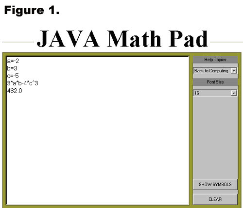
Example 1 Entering and Evaluating Mathematical Expressions
Evaluate the expression 3ab - 4c3 when
a = -2, b = 3, and c = -5.
Solution
Begin by assigning values to the variables. On the Math Pad screen,
type a = -2, then press enter;
type b = 3, then press enter;
type c = -5, then press enter;
Next we type the expression using * to indicate multiplication and
^ for exponents and press enter. Java Math Pad will return the numerical
value of our expression. See Figure 1.
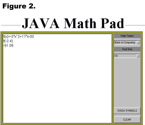
Example 2 Defining and Evaluating Functions
Evaluate the function f(x) = -3x2 + 17x - 33 when x = -2.4
Solution
Click on the Clear button to clear the Java Math Pad screen. Then type f(x)=-3*x^2+17*x-33 and press enter to define the function. Now type f(-2.4) and enter. Java Math Pad will return the value of the function. See Figure 2.
The function f(x) will be stored in Math Pad's memory until clear it. So, you can evaluate the function for as many different values of x as you desire. To clear a defined function from Math Pad's memory type "clear function name". For example, to clear the function f(x) that we just defined, type, "clear f ". You can also simply define a new function named f.
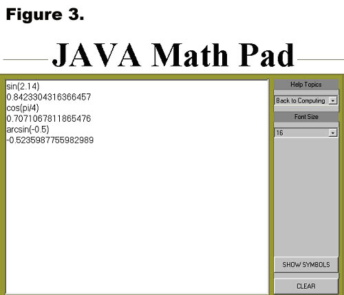
Example 3 Evaluating Trigonometric Functions
Find the value of each of the following trigonometric expressions.
(a) sin(2.14)
(b) cos (π / 4)
(c) arcsin(-0.5)
Solution
The trigonometric and inverse trigonometric functions
are built-in functions in Java Math Pad. In the case of the sine and
cosine functions, the argument must be a number expressed in radians
and must be enclosed in parenthesis. For the inverse sin, the argument
should be a number between -1 and 1 and should also be enclosed in
parenthesis; Math Pad will give the answer in radians. See Figure
3. For more information about the built-in functions, go to "built-in
functions" in Java Math Pad's help menu.
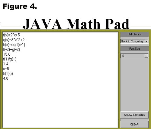
Example 4 Combining Functions to Form a New Function
Given the functions f(x) = 2x + 5, g(x) = 3x2 + 2, and h(x) = √x-1 evaluate each of the following:
(a) f (-2) + g(-2)
(b) f(1) / g(1)
(c) h (f(6))
Solution
Click the Clear button to clear the Math Pad screen. Next define the
three functions. Use sqrt to denote the square root. Type f(x)=2*x+5
and press enter, then type g(x)=3x^2+2 and press enter, and finally
type h(x)=sqrt(x-1) and press enter once again.
(a) Simply type f(-2)+g(-2) and press enter. Math Pad will return
the numerical value.
(b) For this problem, type f(1)/g(1) and press enter.
(c) To evaluate the composite function h(f(x)) when x = 6, you must
first assign the value 6 to the variable x. To do this type x = 6
and press enter. Then type h(f(x)) and press enter. See Figure 4.
Plot-Solve Applet
The purpose of this applet is to plot functions. It
can plot up to 10 different functions at the same time. It can also
be used to solve equations numerically. This demo includes Instructions
for using the applet and examples that will illustrate some of the
features.
1. The Viewing Window Parameters area is used to set the area of the
graph the user wishes to see. Use it as follows:
-
Specify the desired values for XMin, XMax, YMin, YMax. The applet will do basic error checking. If an entry other than a number is typed in, an error will be displayed, and the focus will remain in the field which caused the error.
-
When Use y-range is checked, the supplied values for the y-range will be used. Otherwise, the applet will find YMin and YMax from the supplied functions.
-
Any change in this area will take effect only after the Plot button is pressed.
2. The Function Information area is where
the functions to be plotted are entered. Use this area as follows:
- To enter a new function, always press the New
Function button. Then, enter the expression defining the function.
The syntax is similar to the syntax used in the Java Math Engine.
For example, to defines the sine function, you would type in sin(x).
Make sure you use x for the variable in your definition.
- A maximum of 10 functions can be defined at
the same time.
- Checking Active means the function will show
on the graph. Unselecting it means the function will not show.
- Use the + and - buttons to scroll through the
list of defined functions.
- Each defined function has a different color
assigned to it. The selection is automatic.
- When a function is defined, it is automatically
assigned a name of the form fi where i is a number which starts
at 1 and is incremented every time a new function is defined.
The name a function will be saved under appears to the left of
the field where it is defined.
- Once a function is defined, its name can be
used in the definition of other functions. For example, if two
functions have been defined, the definition of function 3 could
be f1(x)+x*f2(x) Note that we use f1(x) and not just f1.
- The functions defined will plot only after Plot has been pressed.
- Del Function will delete the function currently
showing. When deleting a function, make sure that it is not used
in the definition of another function. An error would occur in
this case. For example, if f2(x) = x + f1(x) and f1 is deleted,
then the definition of f2 contains an unknown symbol, f1.
3. The Zoom and Trace area is where zooming and tracing take place. Use this area as follows:
- To zoom in, picture in your mind the rectangular
region you would like to zoom in. Left click on one of the corners
of this imaginary region. While holding the mouse button down,
move it to the opposite corner, then release it. As you move the
mouse, a rectangle will be drawn to help you visualize the region.
Once the mouse button is released, the graph will redraw, XMin,
XMax, YMin, YMax will be updated.
- To go back to the original view (XMin = -10,
XMax = 10, YMin = -10, YMax = 10), press Reset Zoom.
- To trace, simply single left click in the graph
area. A point will be generated by taking the x-coordinate of
the point where you clicked and the y-coordinate on the function
currently showing.
- To move the point, use the Right or Left buttons.
The point will move on the function currently showing. By selecting
a different function, you can select which function you want your
point to follow.
- The coordinates of the point will be displayed
under X: and Y:.
4. The Control Buttons area contains
buttons which have a global effect for the applet.
- The Clear All button erases all the function
definitions.
- The Plot button is used to update the plot area
after changes in the other areas have been made.
5. The Messages area is where the applet
communicates with the user. Error messages as well as user information
is displayed there. Errors are displayed in red, while information
is displayed in black.
Example 1
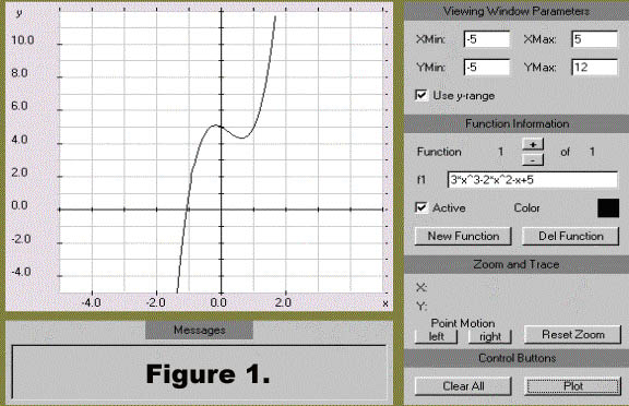
Graph the function f(x) = 3x3 - 2x2 + x + 5.
Solution
Step 1) On the Plot-solve applet, click
the New Function button and type the expression for the function (do
not type f(x)=) using * to indicate multiplication and ^ to indicate
exponents, just as in the Java Math Pad applet.
Step 2) Set the viewing window. The default
window is x-min -10, x-max 10,
y-min -10, y-max 10. You can change these values to give the best
view of the function. In general, you can either specify the y-min
and y-max or you can let the applet choose appropriate y-values for
the function. If you wish to specify the y-min and y-max, "Use
y-Range" must be checked. For this example, set the following
values:
x-min -5, x-max 5, y-min -5, y-max 12.
Step 3) Click the Plot button.
Figure 1 below shows the graph.
Example 2 :
Solve the equation x = x3 + 1 graphically.
Solution
Begin by graphing both the left side and the right side of the equation on the same coordinate axes. To do this, click the New Function button and enter x. Next click New Function again and enter x^3+1. Click the Plot button. The resulting graph is shown in Figure 2. Notice that the default window, x-min -10, x-max 10, y-min -10, y-max 10 gives a good view of the graphs and their point of intersection.
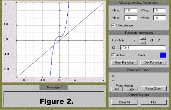
The graph in Figure 2 shows one point of intersection.
The x-coordinates of this point is the solution to the equation. Follow
the steps outlined below to estimate this solution.
Step 1) Place the cursor on the point of intersection and click the left mouse button. The coordinates of the point will appear in the Zoom and Trace portion of the applet. See Figure 3.
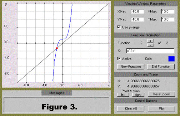
Step 2) Figure 3 shows that the x-value of the point is approximately -1.27. You can get a better estimate of this value by zooming in on the portion of the graph containing that point. To zoom-in on the graph, place the cursor on the graph near the point, but a little to the left and above it; then hold the left mouse button down and drag it to the right and down to form a "box" around the point of intersection. When you are satisfied with the "box", let go of the mouse button and the graph will be redrawn in that viewing window. See Figure 4.
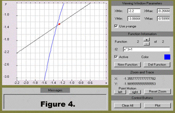
Step 3) Notice that the close-up view shows that we were not actually at the point of intersection. Now move the point closer to the actual point of intersection using the left (or right) button under Point Motion. See Figure 5.
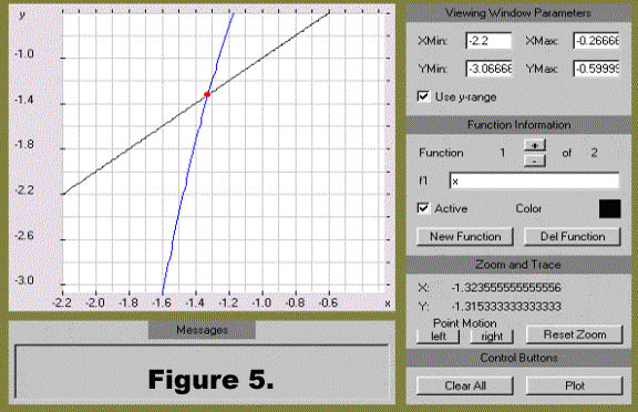
Just as before, the coordinates of the point are displayed by the applet. You can see that a good estimate for the solution to this equation is x = -1.32. You can repeat this procedure as often as necessary to get closer and closer estimates for the point of intersection.
This material is based upon work supported by the National Science Foundation under Grant GEO-0355224. Any opinions, findings, and conclusions or recommendations expressed in this material are those of the authors and do not necessarily reflect the views of the National Science Foundation.